NOT Function – Invert TRUE / FALSE – Excel, VBA, & G Sheets

This tutorial demonstrates how to use the Excel NOT Function in Excel to change TRUE to FALSE or FALSE to TRUE.

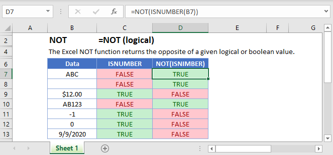
NOT Function Overview

The NOT Function Changes TRUE to FALSE and FALSE to TRUE.

To use the NOT Excel Worksheet Function, select a cell and type:

(Notice how the formula inputs appear)

NOT function Syntax and inputs:

=NOT(logical)

logical – Logical expressions. Example: A1 > 4.

 

What is the NOT Function?

NOT is one of Excel’s logical functions. It reverses the outcome of a logical test. In other words, it checks whether a condition has not been met.

 

How to Use the NOT Function

Use the Excel NOT Function like this:

=NOT(C3="Pop")

Excel will evaluate any logical expression you put in the parentheses, and the return the opposite result. See the example below:

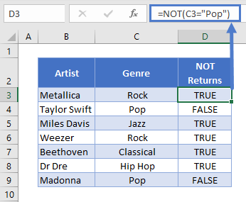
The formula checks whether the genre in column C contains “Pop”. Whatever the result of this test, NOT will flip it.

So, for cells that contain “Pop” (logical test TRUE), NOT returns FALSE. For cells that don’t contain “Pop” (logical test FALSE), NOT flips this to TRUE.

Comparing Text

Note that text comparisons are not case-sensitive. So formula below would return the same results as the above example:

=NOT(C3="POP")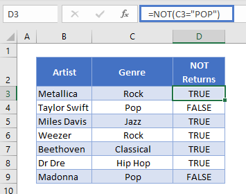

Also, NOT does not support wildcards. So this formula would return TRUE in all cases:

=NOT(C3="P*")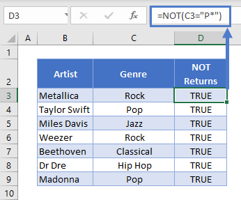

This is because NOT literally compares the text string in C3 with “P*”. Since it doesn’t find that (logical test FALSE), it will return TRUE.

 

Comparing Numbers

When comparing numbers, you can use the following comparison operators:

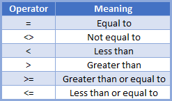
For example, if you had a list of 1980s movies and wanted to exclude ones from 1985 and earlier, you could use this formula:

=NOT(C3<=1985)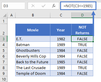

Keep in mind that with NOT, you’re effectively flipping the meaning of these operators. So the above formula is the same as:

=C3>1985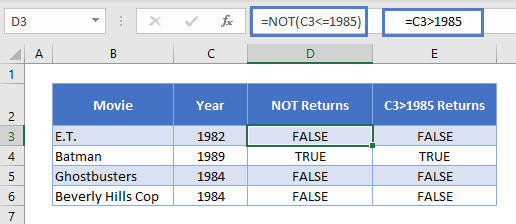

Note also, that if any of the expressions in NOT is, or evaluates to, a non-zero number, NOT will return FALSE:

=NOT(1985)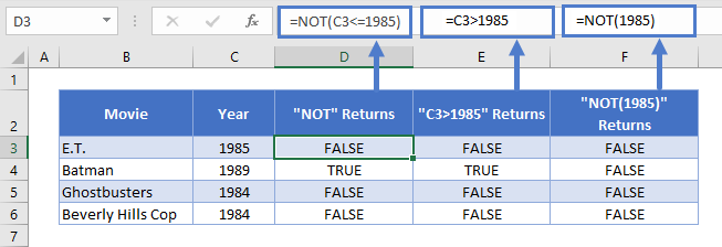

If the expression is, or evaluates to zero, NOT will return TRUE. So these formulas both returns true:

=NOT(1-1)
=NOT(0)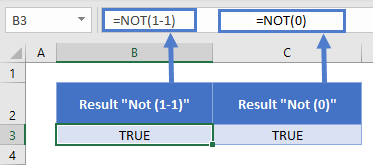

Using NOT with Other Logical Operators

You can combine NOT with any of Excel’s other logical operators, such as AND<<link>>, OR<<link>>, and XOR<<link>>.

For example, say we want to find movies released on or after 1985 that were not directed by Steven Spielberg. We could use this formula:

=AND(C3>=1985,NOT(D3="Steven Spielberg"))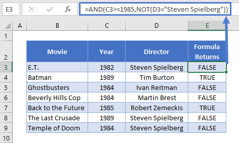

When you combine logical operators like this, Excel evaluates them from the inside-out. So here it will first evaluate the NOT function, and then use its result in the AND.

Using NOT with IF

NOT is most often used within an IF statement. With an IF, instead of just returning TRUE or FALSE after a logical test, you can return whatever you want.

Use it like this:

=IF(AND(C3>=1985,NOT(D3="Steven Spielberg")),"Watch", "Don’t Watch")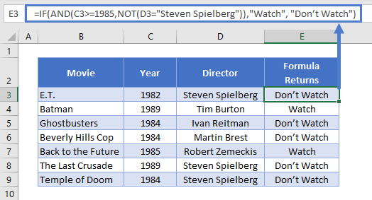

This is the same formula from above, returning TRUE for movies released from 1985 not directed by Spielberg. But now, the IF returns “Watch” if the logical test returns TRUE, and “Don’t watch” if it returns FALSE.

Read more on the main page on the Excel IF Function <<link>>.

NOT in Google Sheets

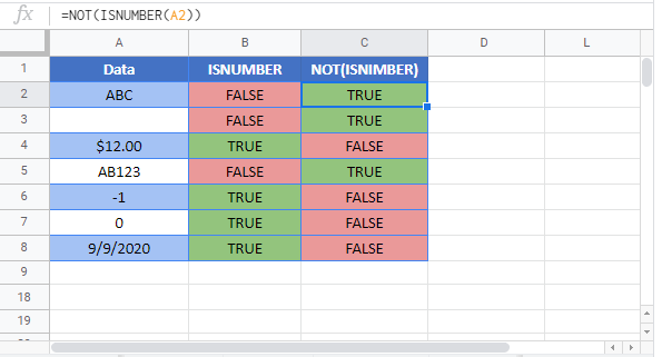
The NOT Function works exactly the same in Google Sheets as in Excel:

Additional Notes

Use the NOT Function to convert TRUE to FALSE and FALSE to TRUE.