MAX Function Examples In Excel, VBA, & Google Sheets

This tutorial demonstrates how to use the Excel MAX Function in Excel to calculate the largest number.

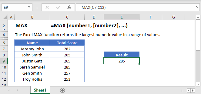
MAX Function Overview

The MAX Function Calculates the largest number.

To use the MAX Excel Worksheet Function, select a cell and type:

(Notice how the formula inputs appear)

MAX function Syntax and inputs:

=MAX(number1,number2)

array – An array of numbers.

How To Use The MAX Function

The MAX Function returns the largest value from a set of data. 

Here let’s use the MAX Function to find the highest GDP in the world:

=MAX(B2:B11)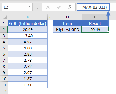

 

Empty Cells or Cells With Text

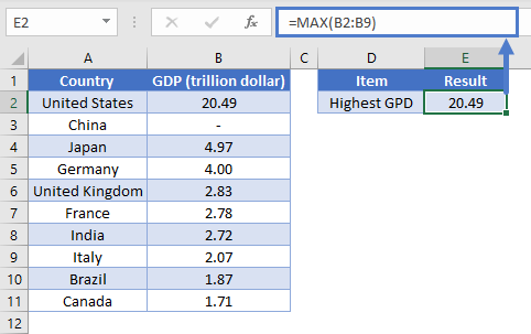
The MAX Function ignores cells that are empty or that contain non-numeric values.

MAX Date

Since Excel stores date as serial numbers, we can use the MAX Function to find the maximum date. 

=MAX(B2:B8)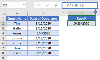

VLOOKUP & MAX

In our above example, we used the MAX Function to determine the highest GDP in the world. After finding the MAX GDP, we can use the VLOOKUP Function to find the country with the highest GDP:

=VLOOKUP(MAX(A2:A9), A2:B9, 2, FALSE)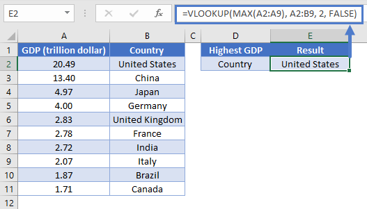

The above function calculates the highest GDP by using the MAX Function. The VLOOKUP Function searches for the highest GDP and returns the information from the second column (as indicated by “2” in our formula) of the search range (A2:B9). 

Note: The item we are looking for (GDP) must be in the first column when using the VLOOKUP Function.

MAXIFS Function

MAXIFS Function returns the maximum value from a data range based on one or more criteria. From our GDP example, suppose we want to find the highest GDP of an Asian country. Use the formula: 

=MAXIFS($C$2:$C$11, $B$2:$B$11, E2)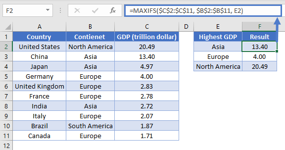

The function narrows down its data range by applying the conditions we provided. It looks for Asia in B2:B11, thus creating a subset from the original data range. The maximum value is then calculated from this subset of data. 

To learn more about how the MAXIFS Function works, read our tutorial on MAXIFS and MINIFS.

Note: MAXIFS Function is only available in Excel 2019 or Excel 365. If you have an older Excel version, you can use Array Function to make your own MAX IF. 

MAX IF 

If you are using older Excel versions, you can combine IF Function with MAX Function using an Array Function. Taking the same example as above, use the formula:

{=MAX(IF(E2=$B$2:$B$11, $C$2:$C$11))}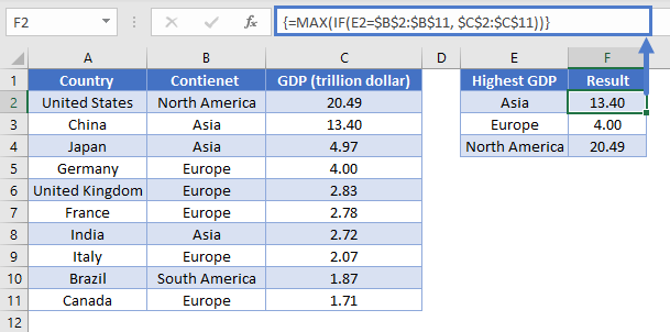

Note: When building array functions, you must press CTRL + SHIFT + ENTER instead of just ENTER after creating your formula.

You’ll notice how the curly brackets appear. You can not just manually type in the curly brackets; you must use CTRL + SHIFT + ENTER.

The formula creates a subset of GDP by using the search criteria. The IF Function searches for “Asia” in B2:B11 and returns the corresponding values from C2:C11 to the MAX Function. Thus, calculating the highest GDP in Asia only. 

Note: The above formula uses absolute references (the $ signs) to lock cell references when copying formulas. If you aren’t familiar with this, please read our Excel References Guide 

 

MAX function in Google Sheets

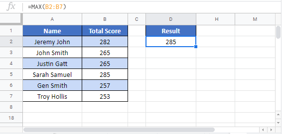
The MAX function works exactly the same in Google Sheets as in Excel.

 

Additional Notes

The MIN Function returns the smallest number in a series.

MAX Examples in VBA

You can also access the Excel MAX Function from within VBA, using Application.WorksheetFunction.

Application.WorksheetFunction.Max(1, 1.23, 3, 21 + 9.43)

The statement above will return 30.43 as the max value (21 + 9.43 = 30.43)

MAX can also accept a range (or Named Range) as a parameter as shown in the VBA code below

Dim Max_Value As Double
Max_Value = Application.WorksheetFunction.Max(Range("A1:A10"))

 

In addition, MAX can accept the name of a table like the one shown above, as a parameter:

Dim Max_Value As Double 
Max_Value = Application.WorksheetFunction.Max(Range("Table1"))

MAX ignores non-numeric values, so the result of the code above is 80.