ERROR.TYPE Function Examples – Excel, VBA, & Google Sheets

This Excel Tutorial demonstrates how to use the Excel ERROR.TYPE Function in Excel to determine the type of error, with formula examples.

ERROR.TYPE Function Description:

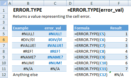
The ERROR.TYPE Function Returns an integer representing the cell error.

Formula Examples:

Example	Formula	Result
#NULL!	=ERROR.TYPE(C5)	1
#DIV/0!	=ERROR.TYPE(C6)	2
#VALUE!	=ERROR.TYPE(C7)	3
#REF!	=ERROR.TYPE(C8)	4
#NAME?	=ERROR.TYPE(C9)	5
#NUM!	=ERROR.TYPE(C10)	6
#N/A	=ERROR.TYPE(C11)	7
Anything else	=ERROR.TYPE(C12)	#N/A

Syntax and Arguments:

The Syntax for the ERROR.TYPE Formula is:

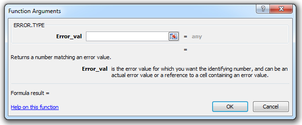
=ERROR.TYPE(error_val)

Function Arguments ( Inputs ):

error_val – The cell reference to an error whose numeric error value you want to obtain.

Additional Notes

Enter the cell reference. <>

How to use the ERROR.TYPE Function in Excel:

To use the AND Excel Worksheet Function, type the following into a cell:
=AND(
After entering it in the cell, notice how the AND formula inputs appear below the cell:

You will need to enter these inputs into the function. The function inputs are covered in more detail in the next section. However, if you ever need more help with the function, after typing “=ERROR.TYPE(” into a cell, without leaving the cell, use the shortcut CTRL + A (A for Arguments) to open the “Insert Function Dialog Box” for detailed instructions:

For more information about the ERROR.TYPE Formula visit the
Microsoft Website.