This tutorial demonstrates how to use the Excel AVERAGE Function in Excel to calculate the average ( mean ).

AVERAGE Function Overview

The AVERAGE Function Averages a series. Text and blank values are ignored. Only numbers are averaged.

To use the AVERAGE Excel Worksheet Function, select a cell and type:

(Notice how the formula inputs appear)

AVERAGE function Syntax and inputs:

=AVERAGE(number1,number2)

array – An array of numbers.

 

What is the AVERAGE Function?

The Excel AVERAGE Function returns the average (arithmetic mean) of a range of values. These values can include numbers, cell references, cell ranges, constants, or arrays.

What is the arithmetic mean?

The arithmetic mean, or just the mean, is the sum of a series of numbers, divided by how many numbers there are in the series.

For example, take the numbers 1,2,3,4,5. We have five numbers in this set, so the mean is:

(1+2+3+4+5) / 5 = 3

How to Use the AVERAGE Function

Use the Excel AVERAGE Function as follows:

=AVERAGE(C3:C9)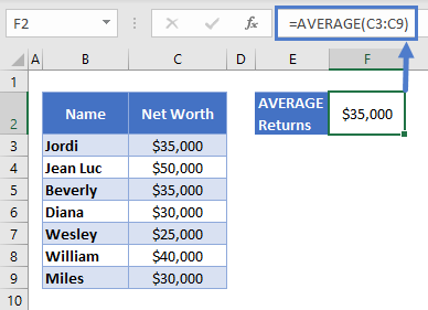

Here we have the net worth of a group of seven work colleagues. AVERAGE calculates their mean net worth at $35,000.

Note that if the data contains any error values at all, AVERAGE will also return an error.

Blanks Vs. Zeros

AVERAGE will ignore any blank cells within the range you define. However, it does include cells containing 0 in the calculation.

In the example below, a new colleague, Reginald, has joined the team, but we don’t know his net worth yet. Since his cell is empty, the mean does not change:

=AVERAGE(C3:C10)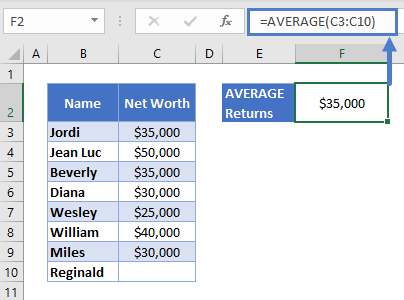

Later, Reginald supplies his net worth, and it turns out he hasn’t saved anything. With 0 in his row, AVERAGE calculates the new mean as shown below:

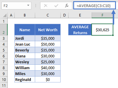
[“Blanks Vs Zero B” screenshot here]

Note that when cells are formatted as a currency, zero values appear as a hyphen, as seen above. That’s only for display purposes, the cell “really” contains a 0.

Extreme Values

The arithmetic mean is useful for data like this, where the numbers are relatively close to each other. If I picked a name from the above group at random, and asked you to guess their net worth as closely as you could, you’d be best off guessing the mean.

However, AVERAGE can give inaccurate estimates if the data contains extreme values.

For example, imagine if the team hired a new employee, Bill Gates:

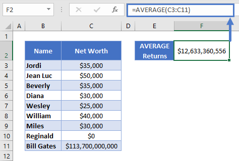
Now the mean doesn’t really represent anyone in the group. If I picked a name again and asked you to guess their net worth, you’d be better off using the previous average, from before Mr. Gates joined the set.

If your data contains extreme values, you may be better off using the MEDIAN Function <<link>> instead.

Creating a Rolling Average

If you have time-series data which contains seasonal fluctuations, it can make the data harder to interpret. One way around this is to create a rolling average.

Let’s say you want to make a 7-day rolling average. To do this:

• Create a new column next to your data called “Rolling Average”
• In your new column, start from the 7^th data point, and use AVERAGE to get the mean of the previous seven days’ data
• Copy the formula down to the bottom of the new column. The cell references will automatically update, giving the mean of the previous seven days each time. See below:

 

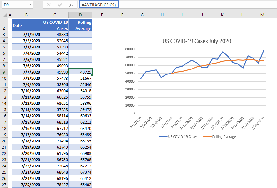
This process is often called “smoothing”, you can see why in the chart below, which shows both the original data and the rolling average. The ups and downs (caused by lower reporting on weekends) are “smoothed out”.

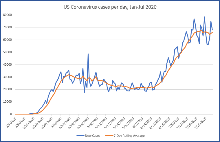
The chart also demonstrates a downside of the rolling average – you miss the first seven days’ data.

 

Use AVERAGEA When You Need to Include Text and Boolean Values

AVERAGEA is similar function, in that it returns the mean of a series of numbers. However, unlike AVERAGE, it includes text and Boolean (TRUE or FALSE) values.

Use it like this:

=AVERAGEA(B3:B9)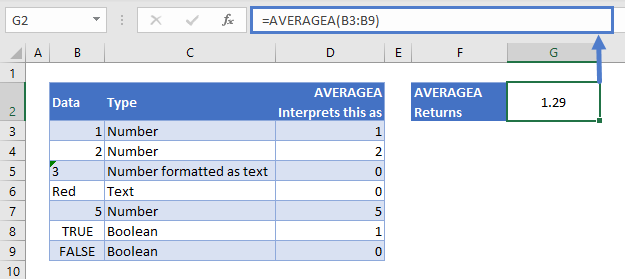

As shown above, AVERAGEA interprets text cells as 0, cells containing TRUE as 1, and cells containing FALSE as 0.

 

Get the Average of the Top Three Scores

Sometimes you might only want to take the average of the highest three numbers within a series. For example, a student’s grade might be calculated based on the mean of their top three exam results.

AVERAGE, when combined with the LARGE Function, can do this for you:

=AVERAGE(LARGE(C3:C8,{1,2,3}))

How this works:

• LARGE accepts a range of values, and returns the nth largest one. The numbers 1, 2, and 3 inside the braces mean we want the 1^st, 2^nd, and 3^rd If you wanted the top five, you’d just add 4 and 5 in here too.
• AVERAGE then returns the mean of these three values

You can see it at work below:

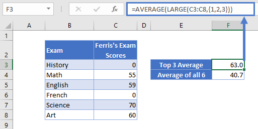
Here we have a student, Ferris, who scored 0 on two exams (he presumably skipped one of the exam days). But since his grade is calculated based on his top 3 exam scores, he still managed to get 63% overall, instead of 40.7%, the average of all 6 results.

 

AVERAGE in Google Sheets

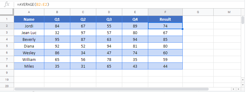
The AVERAGE Function works exactly the same in Google Sheets as in Excel:

AVERAGE Examples in VBA

You can also use the AVERAGE function in VBA. Type:
application.worksheetfunction.average(number1,number2)
For the function arguments (array, etc.), you can either enter them directly into the function, or define variables to use instead.